Getting Started with RStudio
Many Roads to Success!
When first learning to code in R students often feel like there is exactly one way to get to a desired result. One way to load data, one way to draw a density plot, one way to run a regression—this is (emphatically) not true! In almost every case, there are multiple perfectly legitimate ways to conduct an analysis and generate the output you seek, which is great news for a new student! When you have a limited knowledge of R, it is easy to think of coding as a collection of very discrete tasks, where you have one set of functions and syntax to make a scatterplot, and a totally different set of functions and syntax to import data or run a regression. In reality, there is much more similarity between these tasks than difference.
Getting better at R comes from letting yourself experiment with your coding strategy, learning where you can apply techniques from other applications. This may seem confusing right now—that’s fine! This document is intended to get you up to speed with the basics of R and to illustrate how much freedom you have in conducting analyses with RStudio.
Packages
One of the reasons RStudio has so many different overlapping approaches to problems is because of packages. A package is a library of functions that you install and load to extend RStudio’s functionality. A function which is not part of an external package is said to be part of base-R, that is that it comes built in to R by default. Without a doubt, the most important package is tidyverse, a collection of smaller packages that improve on every aspect of base-R, from loading data, cleaning data, visualizing data, etc. tidyverse was first published in 2013, so older RScripts are likely not to make use of the package—which is evidenced by the complexity (and length) of their code.
Writing a script
Project Directory
Before you start coding, you need to create a new project directory. A .proj file simply tells RStudio to start looking for files from whichever directory your .proj file is in—it’s the equivalent of using the setwd(...) function at the top of a script, but you only have to do it one time, even if you have multiple scripts that you’re working in. The other benefit, is that you can share the project directory with an instructor or colleague and your code will function perfectly. If you set a working directory, the person to whom you share a script will have to manually set their own working directory, which can be frustrating, inefficient, and error-prone. It’s a good habit to always work in a project environment.
See the screenshots below to set up your project.
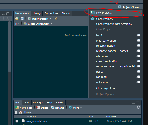
Creating a new project
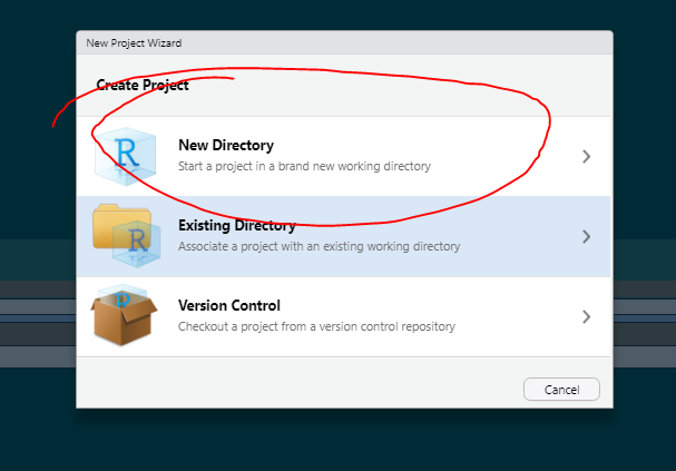
Place the project in a new directory
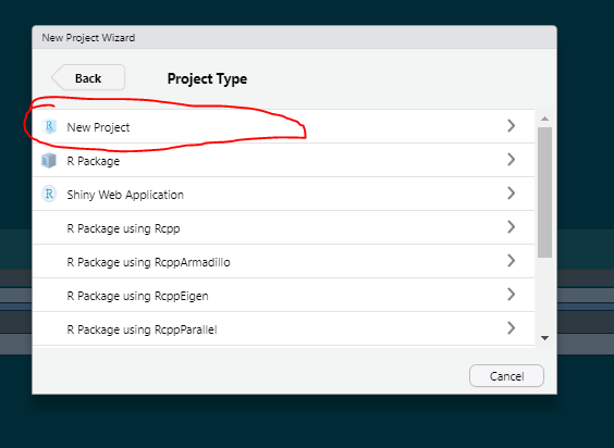
We just need a regular project

Give your project a name, and tell RStudio where to put it
Congratulations! You now have a new project open, but you need to make a new script so you can actually write some code! Click the new script button in the upper left, then save the script (ctrl-s on Windows or cmd-s on a Mac), givign it a descriptive name. Your script is in the upper-left quadrant of your RStudio window and it is where you will write the bulk (if not all) of your code. If you want code to be saved you must write it in your script, not the console or terminal window below.
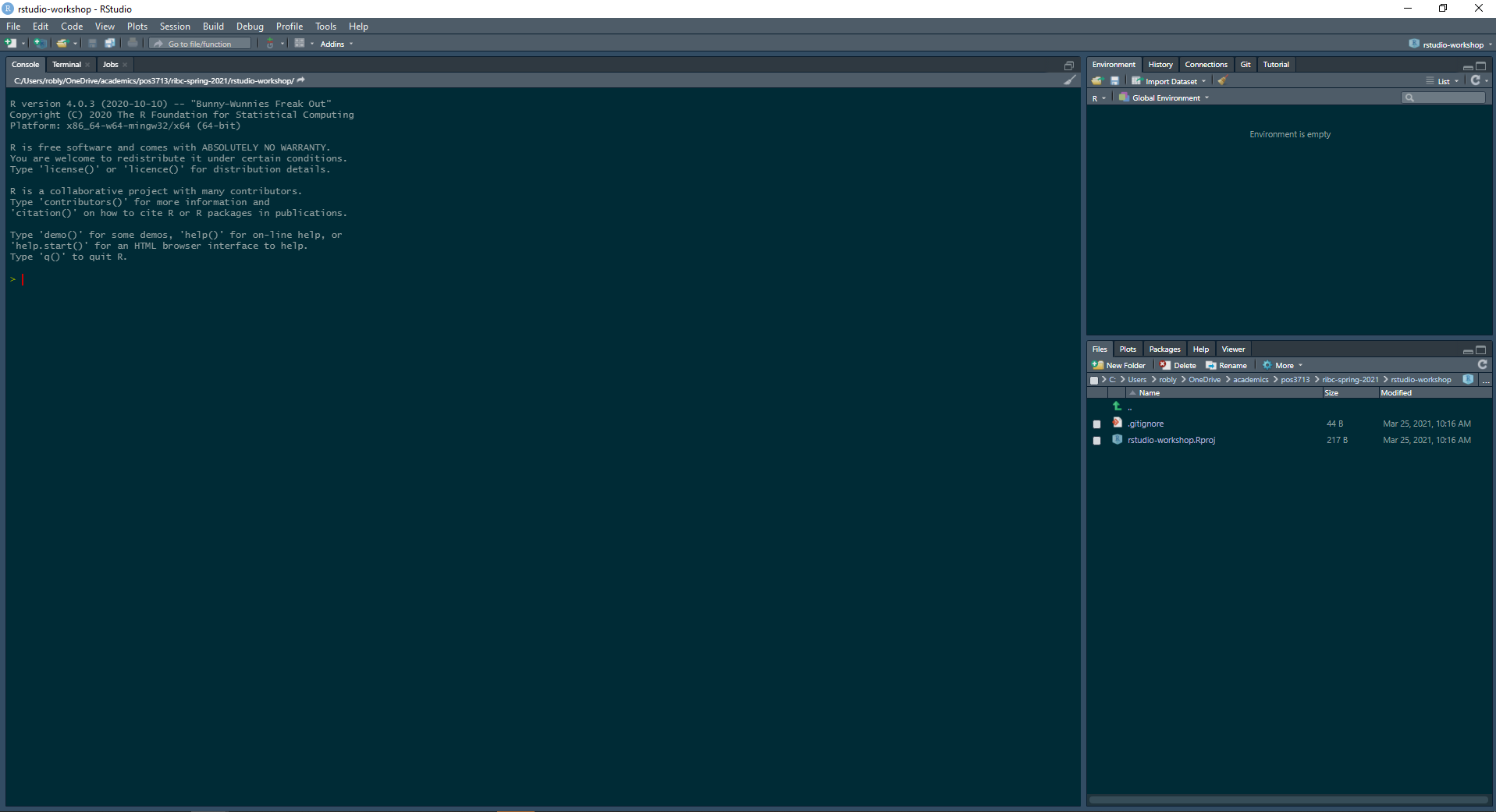
“Click the "new script" button in the upper left corner”
Load packages
Now that we have a script, we can load our packages, this is done with the library() function. Here we are loading tidyverse and haven. haven is a small package that lets us read Stata datasets (.dta). If you don’t have these installed you can do so by installing them through the “Packages” tab in the bottom right of the screen (as in the screenshots below) or by typing install.packages(c("tidyverse", "haven")) in the console. You only need to install packages once; but you need to load them every time you start RStudio.
#Loading packages
library(tidyverse) #We will load tidyverse in every single R script we write. It is invaluable
library(haven) #Haven contains the read_dta() function; this allows us to read Stata (.dta) files
## Warning: package 'haven' was built under R version 4.0.4library(ggeffects) #ggeffects contains useful functions for calculating and plotting predicted valuesYou might get a warning that one or more of your packages was built under a different version of R. This is probably not an issue and you shouldn’t worry about it!
Load your data
To load data in R, it needs to be in a dataframe—an object made up of columns (variables) and rows (observations). We do this by using a function to read the dataset from your computer and the <- operator to put the data into the dataframe:
states_df <- read_dta("data/states.dta") #You can say this as "states_df gets states.dta. i

glimpse(states_df) #take a quick peek at your data, make sure it looks how you expect## Rows: 50
## Columns: 137
## $ state <chr> "Alabama", "Alaska", "Arizona", "Arkansas", "Califor~
## $ state_abbr <chr> "AL", "AK", "AZ", "AR", "CA", "CO", "CT", "DE", "FL"~
## $ gundeath_rate16 <dbl> 21.5, 23.3, 5.0, 17.8, 7.9, 14.3, 4.6, 11.0, 12.6, 1~
## $ gun_murder10 <dbl> 2.8, 2.7, 3.6, 3.2, 3.4, 1.3, 2.7, 4.2, 3.8, 3.9, 0.~
## $ Abort_rank3 <dbl+lbl> 2, 3, 1, 1, 3, 2, 3, 2, 2, 1, 3, 2, 3, 1, 3, 1, ~
## $ Abortion_rank12 <dbl> 20, 35, 5, 4, 49, 25, 45, 30, 26, 9, 42, 22, 36, 7, ~
## $ Adv_or_more <dbl> 7.7, 9.0, 9.3, 6.1, 10.7, 12.7, 15.5, 11.4, 9.0, 9.9~
## $ BA_or_more <dbl> 22.0, 26.6, 25.6, 18.9, 29.9, 35.9, 35.6, 28.7, 25.3~
## $ Cig_tax12 <dbl> 0.425, 2.000, 2.000, 1.150, 0.870, 0.840, 3.400, 1.6~
## $ Cig_tax12_3 <dbl+lbl> 1, 3, 3, 2, 2, 2, 3, 2, 2, 1, 3, 1, 3, 2, 2, 1, ~
## $ Conserv_advantage <dbl> 36.0, 21.3, 19.5, 26.7, 6.3, 15.7, 1.8, 6.3, 17.2, 2~
## $ Conserv_public <dbl> 44.7, 43.1, 36.0, 45.2, 30.8, 36.9, 27.4, 32.3, 36.8~
## $ Dem_advantage <dbl> -14.6, -12.2, -3.5, -1.4, 14.9, -2.4, 17.0, 15.9, 4.~
## $ Govt_worker <dbl> 17.5, 28.0, 15.5, 17.6, 14.9, 15.7, 15.9, 16.1, 14.5~
## $ Gun_rank3 <dbl+lbl> 2, 3, 3, 3, 1, 1, 1, 2, 3, 2, 1, 3, 1, 3, 2, 3, ~
## $ Gun_rank11 <dbl> 17, 50, 50, 39, 1, 15, 5, 18, 41, 22, 6, 47, 9, 39, ~
## $ Gun_scale11 <dbl> 14, 0, 0, 4, 81, 15, 58, 13, 3, 8, 50, 2, 35, 4, 7, ~
## $ HR_cons_rank11 <dbl> 151.7143, 200.0000, 155.5714, 132.5000, 274.2885, 16~
## $ HR_conserv11 <dbl> 65.61905, 55.66667, 62.59524, 69.33333, 54.78931, 59~
## $ HR_lib_rank11 <dbl> 277.5714, 228.0000, 269.8571, 295.2500, 152.4038, 26~
## $ HR_liberal11 <dbl> 34.38095, 44.33333, 37.40476, 30.66667, 81.02201, 40~
## $ HS_or_more <dbl> 82.1, 91.4, 84.2, 82.4, 80.6, 89.3, 88.6, 87.4, 85.3~
## $ Obama2012 <dbl> 38.36, 40.81, 44.45, 36.88, 60.19, 51.45, 58.06, 58.~
## $ Obama_win12 <dbl+lbl> 0, 0, 0, 0, 1, 1, 1, 1, 1, 0, 1, 0, 1, 0, 1, 0, ~
## $ Pop2000 <dbl> 4447100, 626932, 5130632, 2673400, 33871648, 4301261~
## $ Pop2010 <dbl> 4779736, 710231, 6392017, 2915918, 37253956, 5029196~
## $ Pop2010_hun_thou <dbl> 47.79736, 7.10231, 63.92017, 29.15918, 372.53956, 50~
## $ Popchng0010 <dbl> 332636, 83299, 1261385, 242518, 3382308, 727935, 168~
## $ PopchngPct <dbl> 7.5, 13.3, 24.6, 9.1, 10.0, 16.9, 4.9, 14.6, 17.6, 1~
## $ Pot_policy <dbl+lbl> 2, 3, 3, 0, 4, 4, 4, 3, 1, 0, 3, 0, 1, 0, 1, 0, ~
## $ ProChoice <dbl> 36, 58, 56, 40, 65, 61, 68, 63, 58, 52, 57, 41, 58, ~
## $ ProLife <dbl> 54, 37, 39, 55, 28, 34, 26, 31, 36, 43, 35, 55, 33, ~
## $ Relig_Cath <dbl> 6.6, 14.6, 27.3, 5.9, 31.9, 21.9, 41.5, 25.6, 25.4, ~
## $ Relig_Prot <dbl> 79.3, 50.0, 43.3, 78.6, 37.8, 46.1, 32.1, 52.0, 51.2~
## $ Relig_high <dbl> 55.7, 31.3, 36.6, 52.3, 34.5, 33.5, 30.5, 35.2, 37.6~
## $ Relig_low <dbl> 14.3, 39.5, 33.9, 18.7, 36.6, 39.3, 40.4, 33.7, 30.7~
## $ Religiosity3 <dbl+lbl> 3, 1, 2, 3, 1, 1, 1, 2, 2, 3, 1, 3, 2, 2, 2, 3, ~
## $ Romney2012 <dbl> 60.55, 54.80, 53.48, 60.57, 37.09, 46.09, 40.72, 39.~
## $ Smokers12 <dbl> 25, 24, 21, 26, 15, 20, 18, 21, 21, 21, 16, 18, 21, ~
## $ StateID <chr> "AL", "AK", "AZ", "AR", "CA", "CO", "CT", "DE", "FL"~
## $ TO_0812 <dbl> -2.9, -9.4, -3.1, -2.9, -6.5, 0.5, -6.3, -3.5, -4.0,~
## $ Uninsured_pct <dbl> 18.8, 21.8, 20.5, 21.9, 23.2, 17.1, 9.9, 9.6, 22.8, ~
## $ abort_rate05 <dbl> 11.9, 13.6, 16.0, 8.3, 27.1, 16.1, 23.6, 28.8, 26.8,~
## $ abort_rate08 <dbl> 12.0, 12.0, 15.2, 8.7, 27.6, 15.7, 24.6, 40.0, 27.2,~
## $ abortlaw3 <dbl+lbl> 2, 1, 2, 3, 1, 1, 1, 1, 2, 3, 1, 3, 2, 3, 2, 2, ~
## $ abortlaw10 <dbl> 8, 5, 6, 9, 4, 4, 4, 5, 7, 9, 2, 9, 6, 10, 6, 8, 7, ~
## $ alcohol <dbl> 2.01, 3.02, 2.31, 1.83, 2.33, 2.68, 2.34, 3.13, 2.61~
## $ attend_pct <dbl> 52, 22, 29, 50, 33, 29, 30, 35, 35, 45, 35, 45, 39, ~
## $ battle04 <dbl+lbl> 0, 0, 0, 0, 0, 1, 0, 0, 1, 0, 0, 0, 0, 0, 1, 0, ~
## $ blkleg <dbl> 25, 2, 1, 11, 5, 4, 7, 5, 14, 21, 1, 0, 16, 7, 2, 4,~
## $ blkpct04 <dbl> 26.4, 3.6, 3.5, 15.8, 6.8, 4.1, 10.1, 20.4, 15.7, 29~
## $ blkpct08 <dbl> 26.4, 4.3, 4.2, 15.8, 6.7, 4.3, 10.3, 20.9, 15.9, 30~
## $ blkpct10 <dbl> 26.8, 4.7, 5.0, 16.1, 7.2, 5.0, 11.3, 22.9, 17.0, 31~
## $ bush00 <dbl> 56.48376, 58.62096, 51.02114, 51.30720, 41.65137, 50~
## $ bush04 <dbl> 62.46, 61.07, 54.83, 54.31, 44.36, 51.71, 43.95, 45.~
## $ carfatal <dbl> 24.9, 17.4, 20.3, 25.6, 12.1, 17.3, 10.1, 15.0, 19.1~
## $ carfatal07 <dbl> 25.9, 15.2, 17.6, 23.7, 11.7, 12.3, 8.7, 13.6, 18.1,~
## $ cig_tax <dbl> 0.425, 2.000, 2.000, 0.590, 0.870, 0.840, 2.000, 1.1~
## $ cig_tax_3 <dbl+lbl> 1, 3, 3, 1, 2, 2, 3, 2, 1, 1, 3, 1, 2, 2, 2, 2, ~
## $ cigarettes <dbl> 9.41, 6.22, 2.40, 8.51, 3.69, 5.86, 5.47, 17.12, 6.7~
## $ college <dbl> 21.1, 26.7, 24.3, 19.1, 29.1, 34.7, 34.6, 27.6, 25.1~
## $ conpct_m <dbl> 40.67797, 36.32479, 33.33333, 38.87755, 28.46612, 32~
## $ cons_hr06 <dbl> 77.71429, 72.00000, 69.00000, 56.25000, 37.33962, 63~
## $ cons_hr09 <dbl> 72.00, 75.00, 49.50, 28.50, 35.09, 30.29, 1.60, 56.0~
## $ cook_index <dbl> -13.2, -13.4, -6.1, -8.8, 7.4, -0.2, 7.1, 7.0, -1.8,~
## $ cook_index3 <dbl+lbl> 1, 1, 2, 1, 3, 2, 3, 3, 2, 2, 3, 1, 3, 2, 2, 1, ~
## $ defexpen <dbl> 1757, 3556, 1771, 530, 1106, 1139, 2453, 690, 938, 1~
## $ demHR11 <dbl> 14.28571, 0.00000, 28.57143, 25.00000, 64.15094, 42.~
## $ dem_hr09 <dbl> 42.85714, 0.00000, 62.50000, 75.00000, 64.15094, 71.~
## $ demnat06 <dbl> 22.22222, 0.00000, 20.00000, 83.33333, 63.63636, 44.~
## $ dempct_m <dbl> 38.87628, 26.14108, 31.93651, 43.06358, 41.29714, 29~
## $ demstate06 <dbl> 60.71429, 43.33333, 44.44444, 75.55556, 60.83333, 59~
## $ demstate09 <dbl> 57.85714, 46.66667, 41.11111, 72.59259, 64.16667, 59~
## $ demstate13 <dbl> 35.71429, 36.66667, 41.11111, 46.66667, 66.66667, 55~
## $ density <dbl> 94.4, 1.2, 56.3, 56.0, 239.1, 48.5, 738.1, 460.8, 35~
## $ division <dbl+lbl> 6, 9, 8, 7, 9, 8, 1, 5, 5, 5, 9, 8, 3, 3, 4, 4, ~
## $ earmarks_pcap <dbl> 38.9, 425.5, 20.9, 26.7, 12.5, 22.5, 14.8, 25.7, 14.~
## $ evm <dbl> 9, 3, 10, 6, 0, 0, 0, 0, 0, 15, 0, 4, 0, 0, 0, 6, 8,~
## $ evo <dbl> 0, 0, 0, 0, 55, 9, 7, 3, 27, 0, 4, 0, 21, 11, 7, 0, ~
## $ evo2012 <dbl> 0, 0, 0, 0, 55, 9, 7, 3, 29, 0, 4, 0, 20, 0, 6, 0, 0~
## $ evr2012 <dbl> 9, 3, 11, 6, 0, 0, 0, 0, 0, 16, 0, 4, 0, 11, 0, 6, 8~
## $ gay_policy <dbl+lbl> 4, 3, 3, 4, 2, 2, 1, 3, 4, 4, 2, 4, 2, 3, 1, 4, ~
## $ gay_policy2 <dbl+lbl> 1, 1, 1, 1, 0, 0, 0, 1, 1, 1, 0, 1, 0, 1, 0, 1, ~
## $ gay_policy_con <dbl+lbl> 1, 0, 0, 1, 0, 0, 0, 0, 1, 1, 0, 1, 0, 0, 0, 1, ~
## $ gay_support <dbl> 44, 56, 58, 44, 64, 61, 65, 60, 57, 51, 62, 47, 60, ~
## $ gay_support3 <dbl+lbl> 1, 2, 2, 1, 3, 3, 3, 2, 2, 1, 3, 1, 2, 2, 2, 2, ~
## $ gb_win00 <dbl+lbl> 1, 1, 1, 1, 0, 1, 0, 0, 1, 1, 0, 1, 0, 1, 0, 1, ~
## $ gb_win04 <dbl+lbl> 1, 1, 1, 1, 0, 1, 0, 0, 1, 1, 0, 1, 0, 1, 1, 1, ~
## $ gore00 <dbl> 41.56650, 27.66634, 44.73459, 45.86426, 53.44957, 42~
## $ gun_check <dbl> 9024.683, 12016.091, 5313.863, 8443.070, 3040.222, 8~
## $ gun_dealer <dbl> 47.36663, 139.25047, 45.44731, 67.42302, 21.60307, 5~
## $ gun_rank_rev <dbl> 30, 6, 13, 13, 48, 32, 46, 38, 13, 16, 41, 13, 41, 1~
## $ gunlaw_rank <dbl> 19, 43, 36, 36, 1, 17, 3, 11, 36, 33, 8, 36, 8, 31, ~
## $ gunlaw_rank3_rev <dbl+lbl> 2, 1, 1, 1, 3, 3, 3, 3, 1, 2, 3, 1, 3, 2, 3, 2, ~
## $ gunlaw_scale <dbl> 15, 4, 6, 6, 79, 16, 54, 22, 6, 7, 43, 6, 28, 8, 16,~
## $ hispanic04 <dbl> 2.2, 4.9, 28.0, 4.4, 34.7, 19.1, 10.6, 5.8, 19.0, 6.~
## $ hispanic08 <dbl> 2.9, 6.1, 30.1, 5.6, 36.6, 20.2, 12.0, 6.8, 21.0, 8.~
## $ hispanic10 <dbl> 3.9, 5.5, 29.6, 6.4, 37.6, 20.7, 13.4, 8.2, 22.5, 8.~
## $ indpct_m <dbl> 29.96595, 43.56846, 29.71429, 35.93449, 25.82884, 37~
## $ kerry04 <dbl> 36.84, 35.52, 44.37, 44.55, 54.31, 47.04, 54.31, 53.~
## $ libpct_m <dbl> 16.82809, 17.94872, 19.23584, 16.83673, 24.20596, 21~
## $ mccain08 <dbl> 60.32, 59.42, 53.39, 58.72, 36.91, 44.71, 38.22, 36.~
## $ modpct_m <dbl> 42.49395, 45.72650, 47.43083, 44.28571, 47.32791, 45~
## $ nader00 <dbl> 1.0996404, 10.0668861, 2.9794075, 1.4559857, 3.81827~
## $ obama08 <dbl> 38.74, 37.89, 44.91, 38.86, 60.94, 53.66, 60.59, 61.~
## $ obama_win08 <dbl+lbl> 0, 0, 0, 0, 1, 1, 1, 1, 1, 0, 1, 0, 1, 1, 1, 0, ~
## $ over64 <dbl> 13.2, 6.4, 12.7, 13.8, 10.7, 9.8, 13.5, 13.1, 16.8, ~
## $ permit <dbl> 27.6, NA, 46.2, 21.1, 52.8, 46.3, 45.3, NA, 37.8, 27~
## $ pop_18_24 <dbl> 10.004388, 11.144578, 9.614413, 10.075567, 9.952397,~
## $ pop_18_24_10 <dbl> 10.020921, 10.563380, 9.903004, 9.739369, 10.530413,~
## $ prcapinc <dbl> 27795, 34454, 28442, 25725, 35019, 36063, 45398, 358~
## $ region <dbl+lbl> 3, 4, 4, 3, 4, 4, 1, 3, 3, 3, 4, 4, 2, 2, 2, 2, ~
## $ relig_import <dbl> 58.47953, NA, 33.20000, 53.13433, 28.78619, 26.08696~
## $ religiosity <dbl> -13, -177, -140, -23, -147, -163, -170, -109, -84, -~
## $ reppct_m <dbl> 31.15778, 30.29046, 38.34921, 21.00193, 32.87402, 32~
## $ rtw <dbl+lbl> 1, 0, 1, 1, 0, 0, 0, 0, 1, 1, 0, 1, 0, 0, 1, 1, ~
## $ secularism <dbl> 13, 177, 140, 23, 147, 163, 170, 109, 84, 39, 101, 7~
## $ secularism3 <dbl+lbl> 1, 3, 3, 1, 3, 3, 3, 2, 2, 1, 2, 2, 2, 1, 2, 1, ~
## $ seniority_sen2 <dbl+lbl> 0, 1, 0, 0, 0, 0, 0, 0, 0, 0, 0, 0, 0, 0, 0, 0, ~
## $ south <dbl+lbl> 1, 0, 0, 1, 0, 0, 0, 1, 1, 1, 0, 0, 0, 0, 0, 0, ~
## $ to_0004 <dbl> 4.20, -12.39, -2.32, 3.31, 6.63, 0.82, 4.47, 2.53, 8~
## $ to_0408 <dbl> 4.6, -0.8, 1.9, -0.2, 2.9, 3.1, 2.2, 2.0, 3.1, 5.2, ~
## $ trnout00 <dbl> 50.59, 67.19, 44.64, 46.93, 54.61, 57.55, 60.86, 57.~
## $ trnout04 <dbl> 54.79, 54.80, 42.32, 50.24, 61.24, 58.37, 65.33, 59.~
## $ unemploy <dbl> 5.8, 7.5, 5.1, 5.9, 6.2, 5.4, 4.9, 3.9, 4.6, 4.7, 3.~
## $ union04 <dbl> 9.7, 20.1, 6.3, 4.8, 16.5, 8.4, 15.3, 12.4, 6.0, 6.4~
## $ union07 <dbl> 9.5, 23.8, 8.8, 5.4, 16.7, 8.7, 15.6, 12.0, 5.9, 4.4~
## $ union10 <dbl> 10.9, 22.3, 6.5, 4.2, 17.2, 7.0, 17.3, 11.9, 5.8, 4.~
## $ urban <dbl> 55.4, 65.6, 88.2, 52.5, 94.4, 84.5, 87.7, 80.1, 89.3~
## $ vep00_turnout <dbl> 51.6, 68.1, 45.6, 47.9, 55.7, 57.5, 61.9, 59.0, 55.9~
## $ vep04_turnout <dbl> 57.2, 69.1, 54.1, 53.6, 58.8, 66.7, 65.0, 64.2, 64.4~
## $ vep08_turnout <dbl> 61.8, 68.3, 56.0, 53.4, 61.7, 69.8, 67.2, 66.2, 67.5~
## $ vep12_turnout <dbl> 58.9, 58.9, 52.9, 50.5, 55.2, 70.3, 60.9, 62.7, 63.5~
## $ womleg_2007 <dbl> 12.9, 21.7, 34.4, 20.7, 28.3, 35.0, 28.3, 30.6, 23.8~
## $ womleg_2010 <dbl> 12.9, 21.7, 31.1, 23.0, 27.5, 37.0, 31.6, 25.8, 23.1~
## $ womleg_2011 <dbl> 13.6, 23.3, 34.4, 22.2, 28.3, 41.0, 29.9, 25.8, 25.6~
## $ abbr_merge <dbl+lbl> 3, 3, 3, 3, 3, 3, 3, 3, 3, 3, 3, 3, 3, 3, 3, 3, ~Above, we used the function read_dta() from the haven package, because our dataset is a .dta file. If we had a .csv or .rds file, we would use the functions read_csv() or read_rds() from `tidyverse.
You can name your dataframe anything (besides TRUE and FALSE), but try to make it descriptive to you. Since our dataset is called states.dta, I called the dataframe states_df because it is short and descriptive.
Start visualizing your data
Density plots
Let’s make a few density plots of the variable womleg_2011, the proportion of women in the state legislature in the year 2011.
#Here is how you can make a density plot in base-R. I do not recommend this approach, but it is worthwhile learning it to build your understanding or R.
#In your work, you are quite likely to come across older Rscripts which use these functions, and you should know how to read those.
plot(density(states_df$womleg_2011))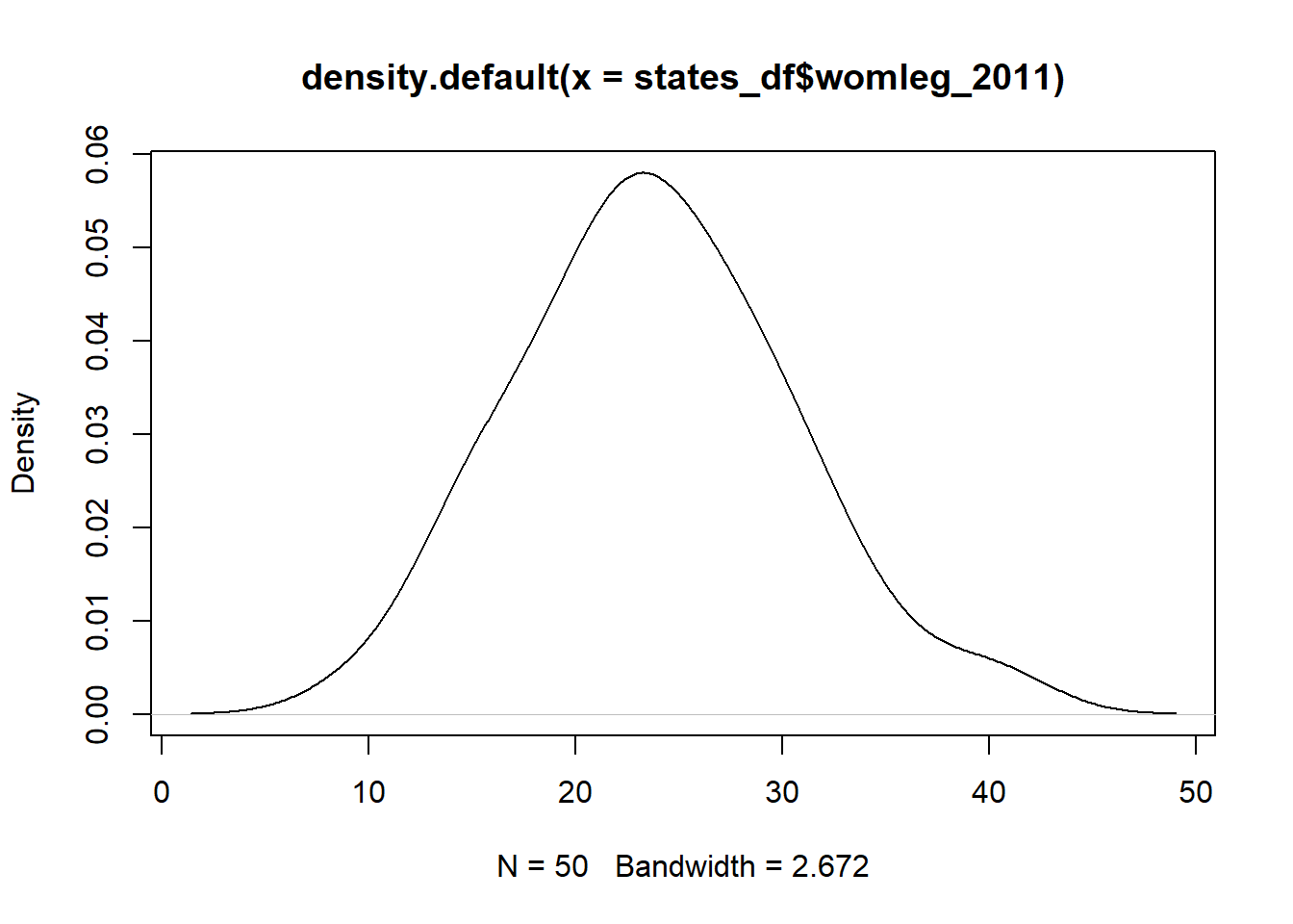
#qplot is a function in the ggplot package that functions similarly to plot() in base-R
#qplot picks the appropriate plot style automatically based on the number and type of variables that you input.
#qplot is handy when you want to get a quick peek at the data, but you're better off using ggplot() if you want to generate a publication quality visual.
qplot(states_df$womleg_2011)
## `stat_bin()` using `bins = 30`. Pick better value with `binwidth`.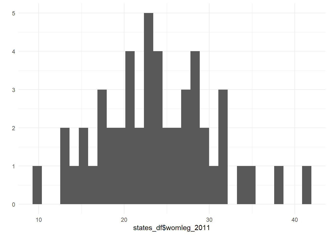
# Here is a density plot of womleg_2011 in ggplot() this probably looks familiar to you from last semester
ggplot(data = states_df, aes(x = womleg_2011)) +
    geom_density()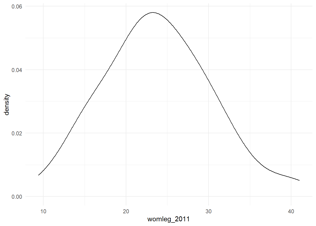
As you can see, these three approaches (plot(), qplot(), and ggplot()) look quite different, but they all generate plots which look about the same. ggplot() is the approach I recommend for almost every application. It’s very easy to extend, customize, and label your plot in ways that are difficult with plot(), or qplot().
Now let’s try making a scatterplot with ggplot(). Here we’re using variables for percent of the legislature who are women and the percentage of unionized workers in the laborforce.
Scatterplot
ggplot(data = states_df, aes(x = union10, y = womleg_2011)) +
    geom_point() +#the geom_point() argument tells ggplot to make a scatterplot with these data
    labs(x = "Percent Workers Unionized (2010)", #adding some nice labels
             y = "Percent of Legislature Women (2011)",
             title = "Unionization and Women's Representation")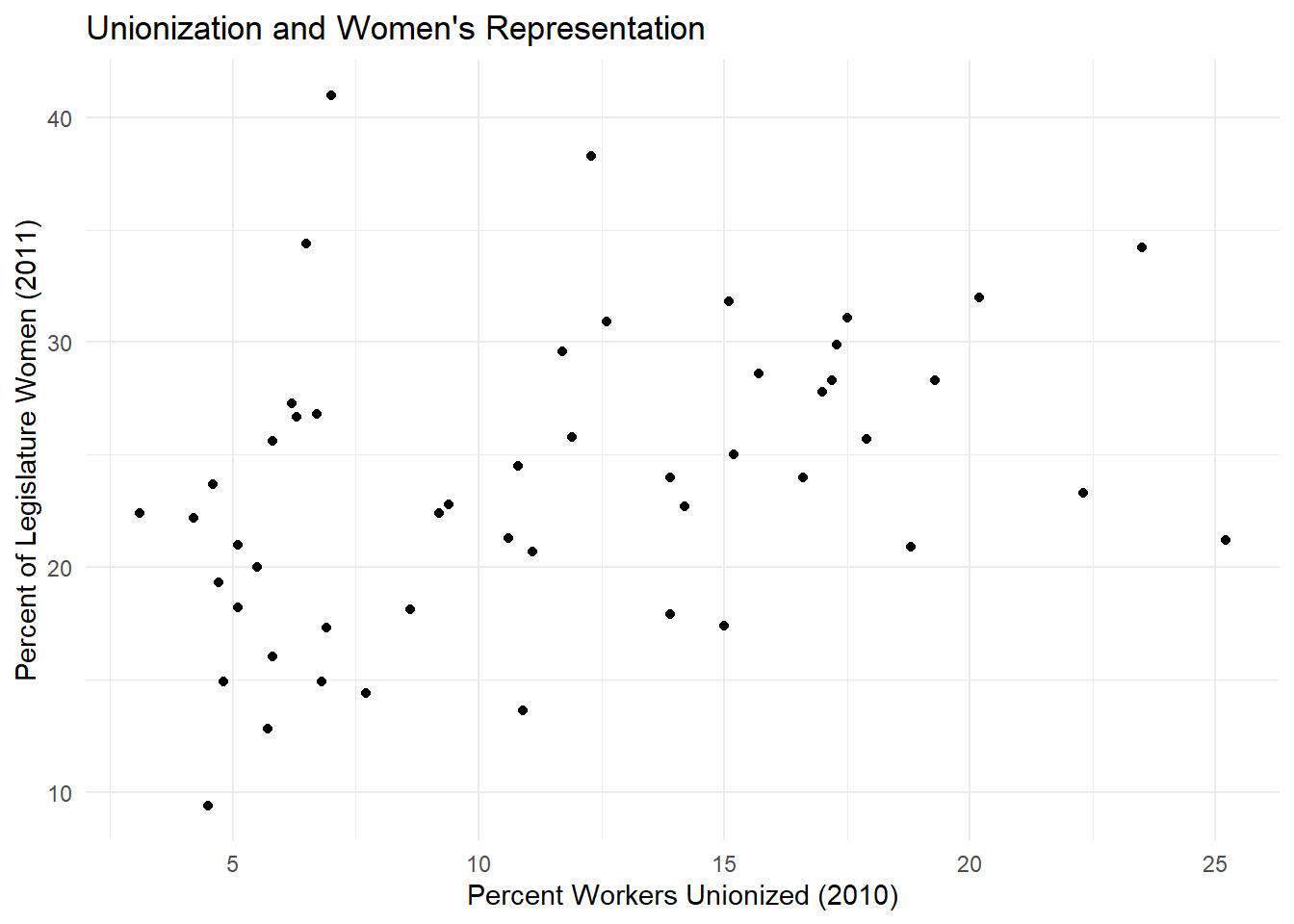
Regression
Taking those same variables, let’s run a bivariate regression analysis. A linear regression is done with the function lm(). The first argument in lm() is the regression formula. Write your dependent (outcome) variable on the left hand side and our independent variable on the right hand side. In place of =, we have to use the ~ in the formula (since = already means something to R).
bv_model <- lm(womleg_2011 ~ union10, data = states_df) #running the regression and putting it in an object
summary(bv_model)##
## Call:
## lm(formula = womleg_2011 ~ union10, data = states_df)
##
## Residuals:
## Min 1Q Median 3Q Max
## -11.5090 -4.6032 -0.3062 4.0011 19.0342
##
## Coefficients:
## Estimate Std. Error t value Pr(>|t|)
## (Intercept) 19.0068 1.9566 9.714 6.49e-13 ***
## union10 0.4227 0.1538 2.749 0.00841 **
## ---
## Signif. codes: 0 '***' 0.001 '**' 0.01 '*' 0.05 '.' 0.1 ' ' 1
##
## Residual standard error: 6.234 on 48 degrees of freedom
## Multiple R-squared: 0.136, Adjusted R-squared: 0.118
## F-statistic: 7.555 on 1 and 48 DF, p-value: 0.008407summary(bv_model) returns lots of useful information about our regression. We see the estimate of the coefficient (the slope of our line). In this case, our coefficient estimate tells us that a one unit increase in union membership is associated with a .4227 unit increase in women’s descriptive representation. We also see the p-value, which tells us the probability of observing a relationship as (or more) extreme than this one by chance. In other words, if the null hypothesis is true, we would expect to find an association as strong or stronger than .4227 about \(.8\%\) of the time. This is a statistically significant result.
#running some predictions. Predicting the percent of women in the legislature at min/max valu
predict(bv_model, data.frame(union10 = min(states_df$union10))) #min() and max() are functions that return the min/max of a variable## 1
## 20.31722predict(bv_model, data.frame(union10 = max(states_df$union10)))## 1
## 29.65922#lets plot this line in our ggplot()
#create a dataframe containing all values of the regression line
bv_predict <- ggemmeans(bv_model, terms = "union10") #Here you use quotation marks around the column. This is an exception to the rule---i'm not sure why!## Loading required namespace: emmeansglimpse(bv_predict)## Rows: 24
## Columns: 6
## $ x <int> 3, 4, 5, 6, 7, 8, 9, 10, 11, 12, 13, 14, 15, 16, 17, 18, 19,~
## $ predicted <dbl> 20.27495, 20.69766, 21.12038, 21.54309, 21.96581, 22.38852, ~
## $ std.error <dbl> 1.5586346, 1.4344500, 1.3165308, 1.2067151, 1.1074163, 1.021~
## $ conf.low <dbl> 17.14110, 17.81351, 18.47332, 19.11683, 19.73920, 20.33425, ~
## $ conf.high <dbl> 23.40879, 23.58182, 23.76744, 23.96936, 24.19242, 24.44280, ~
## $ group <fct> 1, 1, 1, 1, 1, 1, 1, 1, 1, 1, 1, 1, 1, 1, 1, 1, 1, 1, 1, 1, ~glimpse()ing bv_predict, we see several columns. x is simply all the x values at which we have observations and predicted is the estimated y value of the regression line. std.error is the standard error of the estimate. conf.low and conf.high are the upper and lower confidence intervals. We’ll cover group a bit later.
Now, we can add this prediction to our ggplot(), by adding our predicted dataframe to geom_line()! In ggplot(), you can call more than one dataframe by adding the data = ... and aes() arguments to your geom_*. You don’t need to do this too often, but is helpful in this case. If you don’t call data = or aes() in your geometry, the geom_*() argument will simply use whatever data and aesthetics you called initially.
To add your regression line to the scatterplot, you can copy-and-paste your scatterplot code from above and add geom_line(data = bv_predict, aes(x = x, y = predicted)), like so. Remember to add a + to each function except for the last.
ggplot(data = states_df, aes(x = union10, y = womleg_2011)) +
    geom_point() +#the geom_point() argument tells ggplot to make a scatterplot with these data
    geom_line(data = bv_predict, aes(x = x, y  = predicted)) +
    labs(x = "Percent Workers Unionized (2010)", #adding some nice labels
             y = "Percent of Legislature Women (2011)",
             title = "Unionization and Women's Representation")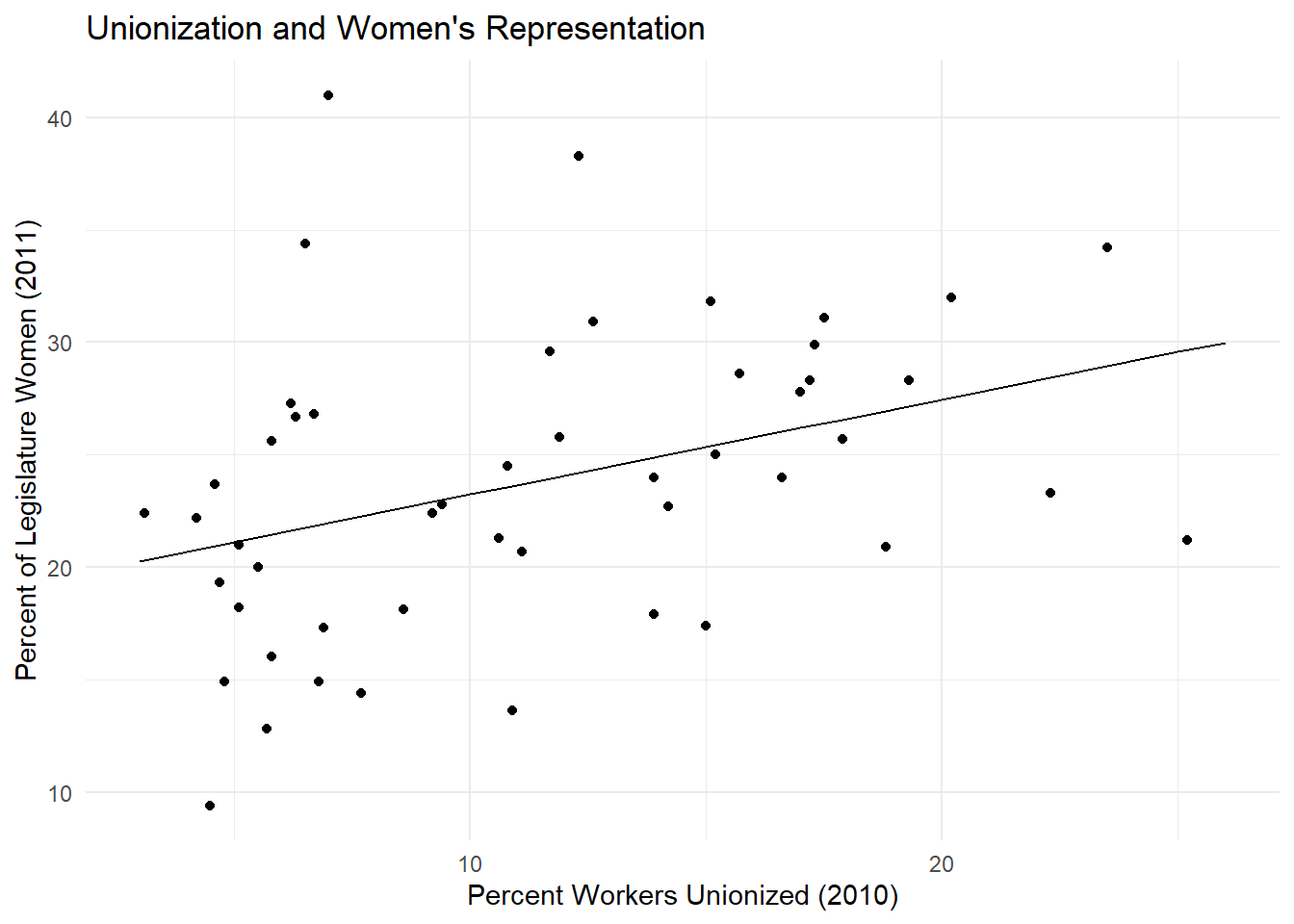
Now let’s do the same thing with a multivariate model. We’ve added a control variable cook_index, which shows states’ partisanship—low values indicate a state is more Republican, high values more Democratic. Using the function ggemmeans() we can estimate the “effect” of union membership on women’s representation at different levels of partisanship. This lets us show the predicted “effect” of x on y at diffent levels of our control variable.
mv_model <- lm(womleg_2011 ~ union10 + cook_index, data = states_df) #run the regression just as before, adding cook_index to your formula
summary(mv_model)##
## Call:
## lm(formula = womleg_2011 ~ union10 + cook_index, data = states_df)
##
## Residuals:
## Min 1Q Median 3Q Max
## -12.1629 -4.0108 -0.3438 2.3514 15.9817
##
## Coefficients:
## Estimate Std. Error t value Pr(>|t|)
## (Intercept) 25.35596 2.26298 11.205 7.19e-15 ***
## union10 -0.03492 0.17146 -0.204 0.839506
## cook_index 0.46614 0.11086 4.205 0.000116 ***
## ---
## Signif. codes: 0 '***' 0.001 '**' 0.01 '*' 0.05 '.' 0.1 ' ' 1
##
## Residual standard error: 5.37 on 47 degrees of freedom
## Multiple R-squared: 0.3722, Adjusted R-squared: 0.3455
## F-statistic: 13.93 on 2 and 47 DF, p-value: 1.776e-05mv_predict <- ggemmeans(mv_model, terms = c("union10", "cook_index")) #since we have two terms we have to wrap them in the c() function. We are giving `ggemmeans()` a list, not a single value
glimpse(mv_predict)## Rows: 72
## Columns: 6
## $ x <int> 3, 3, 3, 4, 4, 4, 5, 5, 5, 6, 6, 6, 7, 7, 7, 8, 8, 8, 9, 9, ~
## $ predicted <dbl> 19.92320, 24.09984, 28.27648, 19.88828, 24.06492, 28.24156, ~
## $ std.error <dbl> 1.3453077, 1.6218310, 2.3289851, 1.2506266, 1.4725254, 2.178~
## $ conf.low <dbl> 17.21679, 20.83713, 23.59116, 17.37234, 21.10258, 23.85894, ~
## $ conf.high <dbl> 22.62961, 27.36254, 32.96179, 22.40422, 27.02726, 32.62417, ~
## $ group <fct> -11.43, -2.47, 6.49, -11.43, -2.47, 6.49, -11.43, -2.47, 6.4~Notice when we glimpse(mv_predict) we get three different values in group. These are different terciles of cook_index, and are calculated automatically by ggemmeans. We can make use of these in our ggplot(), by mapping the color aesthetic to group.
ggplot(data = states_df, aes(x = union10, y = womleg_2011)) +
    geom_point() +#the geom_point() argument tells ggplot to make a scatterplot with these data
    geom_line(data = mv_predict, aes(x = x, y = predicted, color = group)) +
    labs(x = "Percent Workers Unionized (2010)", #adding some nice labels
             y = "Percent of Legislature Women (2011)",
             color = "Cook Index", #titling our legend
             title = "Unionization and Women's Representation")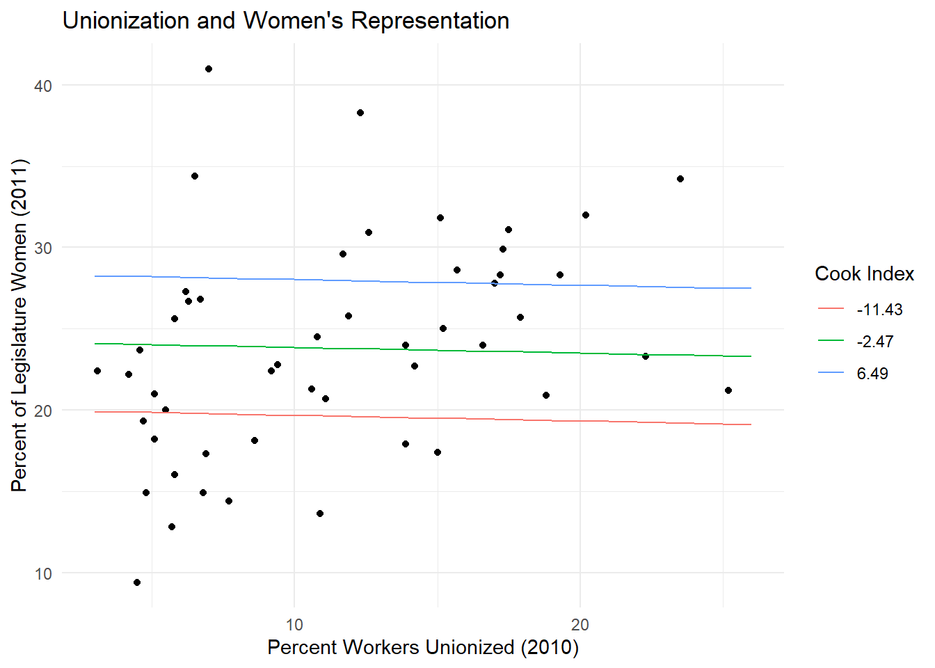
Now, instead of one estimate, we have three—one for each tercile of our partisan cook index control variable. When we control for partisanship, the apparent positive relationship between union membership and women’s representation disappears.